| Contributing Authors: | Sonia Kéfi, Florian Schneider, Alain Danet, Alexandre Génin, Angeles G. Mayor, Susana Bautista, Max Rietkerk, Koen Siteur |
| Editor: | Jane Brandt |
| Source document: | Kéfi, S., Schneider, F. Danet, A., Génin, A. Mayor, A. G., Bautista, S. Rietkerk, M. Siteur, K. 2017. Report on indicators for critical thresholds. CASCADE Project Deliverable 6.2, 26 pp |
1. Generic early warning signals
Theoretical studies have suggested that a number of ‘generic’ indicators could be derived based on a phenomenon that appears to be universal prior to bifurcations (i.e. points at which the stability of a systems changes, such as a tipping point): critical slowing down [27]. Critical slowing down means that the time needed for a system to return to equilibrium following a small disturbance gets longer as the system approaches a bifurcation point (Figure 1b-c). In other words, closer to a bifurcation, the system has a harder time recovering from perturbations, and the capacity of the system to absorb perturbations without shifting to a different state decreases.
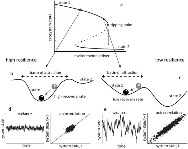
Far from the tipping point resilience is high (b): the ecosystem lies in a steep basin of attraction. Small disturbances are damped by high recovery rates back to equilibrium. Rate to recover from perturbations is high (b), the dynamics are characterized by low variance (d), and low correlation between subsequent states (d). Close to the tipping point resilience is low (c): the ecosystem lies in a less steep basin of attraction. Rate to recover from perturbations is low (c), the dynamics are characterized by high variance (e), and high correlation (e). Figure modified from [28].
Critical slowing down has direct statistical signatures that have led to the definitions of generic early-warning signals of ecosystem degradation [21]. First, critical slowing down can be assessed by measuring the recovery rate of the system upon a disturbance (which should decrease as a system approaches a bifurcation point) [29] (Figure 1b-c). Second, slowing down leads to an increase in variance prior to a tipping point: the state of the ecosystem should fluctuate more widely around its equilibrium [30] (Figure 1d-e). Third, there is an increase in autocorrelation: the state of the ecosystem resembles more its previous state when it is close to a bifurcation point [31] (Figure 1d-e).
The generic early-warning signals have been developed and tested in a number of models (e.g. [32]). In harsh environments such as drylands, recruitment of woody plants often depends on nurse plants that ameliorate stressful conditions and facilitate the establishment of seedlings under their canopy. For example, C. Xu, S. Kéfi and colleagues [33] used an individual-based model and demonstrated that these facilitative interactions may cause a treeless and a woodland state to be alternative stable states on a landscape scale if nurse plant effects are strong and if the environment is harsh enough to make facilitation necessary for seedling survival (Figure 2A). A corollary is that under such conditions, environmental change can bring drylands to tipping points for woody plant encroachment (path 4-3-1 in Figure 2A) or woodland collapse (path 1-2-4 in Figure 2A). We showed that the proximity of tipping points can be announced by the generic early-warning indicators, i.e. by slowness of recovery of woody vegetation cover from small perturbations (because of critical slowing down; Figure 2B, C) as well as by elevated temporal and spatial auto-correlation and variance (Figure 2D-G).
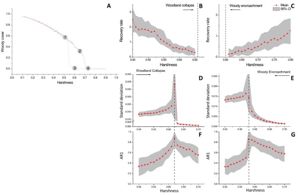
As harshness increases, the woodland collapses catastrophically into a treeless state (path 1-2-4). After a collapse, a decrease in environmental harshness can lead to an abrupt recovery of the woody vegetation following the path 4-3-1. The ecosystem therefore exhibits two tipping points located around point 2 (woodland collapse tipping point) and point 3 (woody encroachment tipping point). B-C: The recovery rate of the ecosystem upon small perturbations slows down towards both tipping points (dashed lines). D-G: Temporal indicators of critical slowing down. Variance (standard deviation, D-E) and temporal correlation (lag-1 autoregressive coefficient, AR1, F-G) in simulated time series rise towards tipping points (dashed lines) for a shift from high to low woody cover (woodland collapse) as well as for a shift from low to high woody cover (woody encroachment). Figure modified from [33].
The genericity of early warning signals. Most studies on the generic early-warning signals had initially focused on models exhibiting tipping points and catastrophic shifts, and it was unclear how these indicators behaved in systems approaching other types of bifurcations. In particular, it was unclear whether the early-warning signals were specific to catastrophic shifts or whether they could also occur in cases of abrupt but reversible ecosystem responses. In CASCADE we tested the behavior of the generic early-warning signals as a model system approached different types of bifurcations [34].
We found that all indicators showed consistent patterns for a variety of bifurcations. In particular, we found that the generic early-warning signals were not specific to catastrophic bifurcations but also preceded non-catastrophic transitions [34]. The generic early-warning signals can generally be detected in situations where a system is slowing down, i.e. becoming increasingly sensitive to external perturbations, independently of whether the impeding change is catastrophic or not.
2. Spatial generic early warning signals: indicators specifically based on spatial information
Studies have shown that slowing down in space takes place in an analogous way to slowing down in time [35,36]. Spatial variance and spatial correlation between near-neighbors are expected to rise as a system is approaching a bifurcation point. However, in models that show a strong spatial structure, like drylands, it has been shown that most of the generic early warning signals can fail [32]. In such cases, indicators specific to those systems need to be developed.
In drylands, vegetation is characterized by spatial patterns formed by the isolated vegetation patches interspersed with bare soil. In addition to the spatial generic early warning signals, studies have suggested that changes in the spatial vegetation patterns themselves could be indicative of environmental deterioration in semi-arid ecosystems [24,26]. In particular, the shape of the vegetation patches [1,37] and the distributions of vegetation patch sizes could indicate that an ecosystem is degrading [25,26].
In CASCADE we reviewed these spatial indicators of ecosystem degradation suggested by the theoretical literature [23] (early-warning signals and patch-based indicators), and we developed a methodological framework for the practical quantification and the interpretation of these indicators on real data (Figure 3).
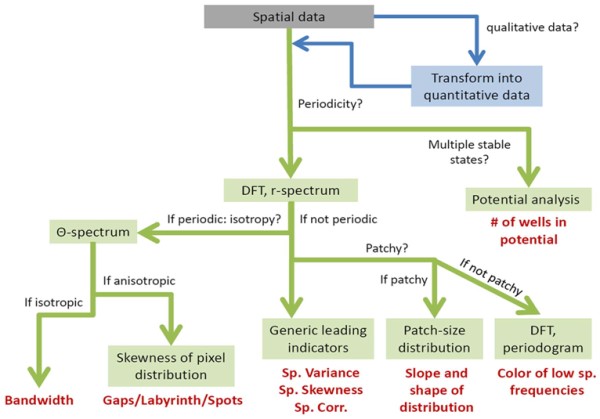
We developed a statistical toolbox in the free programming R environment whose code is freely available online as well as a webpage aiming at describing and explaining the various indicators (in time and space) and their theoretical foundation, giving some concrete examples of case studies and references from the literature (see »Early warning signals toolbox).
3. Refining the understanding and use of indicators
Patch-based indicators and spatial stressors. The theoretical foundations of early warning signs of catastrophic shifts had so far assumed that pressures on ecosystems distribute homogeneously in space. While this may be valid for some pressures, it is most certainly not true for others such as livestock grazing, which is not only a major human supply factor, but also a primary trigger of desertification. In CASCADE we developed a dryland vegetation model including grazing and its spatial component (see »Simulated pressures and ecosystem responses; [8]), and we investigated the behaviour of the spatial indicators of degradation in this model.
Our model analysis shows that spatially-explicit grazing disrupted patch growth and put even apparently 'healthy' drylands under high risk of catastrophic shifts (Figure 4). Our study highlights that the spatial indicators of degradation can fail in ecosystems where the pressure is spatially heterogeneous, such as grazed drylands. Our results may very well generalize to other ecosystems exhibiting self-organized spatial patterns where a spatially-explicit pressure disrupts pattern formation.
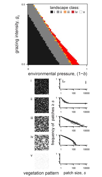
(i: full cover; ii: up-bent power law with spanning clusters; iii: pure power-law; iv: down-bent power law; v: desert) along gradients of environmental and grazing pressures. Note that at high grazing pressure, a vegetation collapse was not preceded by down-bent power laws. Figure adapted from [8].
Periodic patches and patch adaptation in response to environmental changes. CASCADE partners [38] studied a simplified vegetation reaction-diffusion-advection model producing periodic vegetation patterns. Model studies revealed that patterned ecosystems may respond in a non-linear way to environmental changes, meaning that gradual changes can lead to sudden desertification. In Siteur et al. [38] we studied this response through a novel stability analysis of patterned vegetation states. We found that, besides direct critical transitions through decreased rainfall, patterned vegetation states may also adapt, depending on the rate of environmental change and the amount of noise. Rapid environmental change and lack of noise resulted in a drastic critical transition (top right panel), while patterns could adapt in the case of slow environmental change (top left panel). In the model, the vegetation patterns adapted to environmental change in two ways: 1) by adapting biomass while the wave number of the periodic patches remained the same and 2) by adapting wave numbers. We were able to construct so-called ‘Busse balloons’, showing the surface in parameter planes for which stable patterned vegetation states can be found (grey area). These findings shed a more nuanced light on the earlier suggestions that regular patterns in those systems would indicate bistability and proximity to catastrophic shifts [24,37]. Indeed, these model results suggest that ecosystems may adapt and catastrophic shifts may be avoided, if environmental changes are sufficiently slow.
Including rainfall intensity. How annual and seasonal rainfall volumes in arid and semi-arid regions will change in the coming decades is subject to much uncertainty, according to global climate model projections. In contrast, projections of changes in rainfall intensity show strong trends. Rainfall intensity has an important impact on spatial infiltration patterns of water in patchy arid ecosystems [39,40], and it is unknown if and exactly how the projected changes in rainfall intensity are going to affect the productivity and functioning of patterned semiarid ecosystems.
CASCADE partners [41] performed a model analysis to address that question and concluded that projected increases in rainfall intensity could induce and enhance alternative stability of semi-arid ecosystems. We also found that under certain conditions both an increase and a decrease in mean rainfall intensity could push the system over a critical threshold, resulting in a regime shift to a bare desert state. This finding was attributed to the fact that water can be lost from the system in two ways. During high intensity rain events, a fraction of the water flows through the vegetation bands and is lost as runoff, while during low intensity events a large portion of the water infiltrates in the bare interbands, where it is less available to plants and can eventually be lost due to soil evaporation and percolation.
4. Developing new, additional indicators
In addition to the early-warning signals and the patch-based indicators, new indicators were also suggested in CASCADE, which are hereafter presented (see Table 1 for an overview of all these indicators).
Table 1: Table summarizing the different indicators studied in WP6.
| Indicator name | Description | Advantages | Drawbacks | References |
| Cover | Percentage of the ground covered by vegetation | Easy to understand, easy to measure | Fails in the case of ecosystem shift | [18–20] |
| Temporal generic indicators | Temporal variance, auto-correlation at lag 1 and temporal skewness calculated on time series of a variable of the ecosystem state (e.g. cover, abundance of a key species…) | Works independent of the type of changes expected in the ecosystem (i.e. both with continuous degradation and catastrophic shifts) | Requires to use more advanced statistical tools (but tools freely available); Requires detailed time series of the variable | [21,22] |
| Spatial generic indicators | Spatial variance, near-neighbour correlation and spatial skewness calculated on spatial data (e.g. aerial images on which vegetation abundance or presence/absence can be estimated in space) | Works independent of the type of changes expected in the ecosystem; Only a few spatial snapshots in time are required to get an idea of the trend that an ecosystem follows through time | Requires to use more advanced statistical tools (but tools freely available) Requires spatial data or maps with sufficient resolution | [21,23] |
| Patch-based indicators | Metrics quantifying the shapes, sizes, distribution of patch sizes present in the landscape and power law range (PLR, i.e. the proportion of the distribution that fits a power law) | More powerful than generic indicators for patchy landscapes (i.e. landscapes with a strong spatial structure); Works independent of the type of changes expected in the ecosystem | Only works on patchy landscapes; Requires to use more advanced statistical tools (but tools freely available) Requires spatial data or maps with sufficient resolution | [23,25,26,32] |
| Flowlength | Metric quantifying the connectivity of bare-soil areas in the landscape, which is a proxy for how much resource can be lost from the system. | More powerful than cover for patchy landscapes; Works independent of the type of changes expected in the ecosystem | Only works on patchy landscapes; Requires to use more advanced statistical tools | [16,42] |
| Network-based indicators | Metrics calculated on spatial data after transformation them into a network of interaction. In such network the mean and variance of the node degree are followed. | More powerful than generic indicators | Requires to use more advanced statistical tools | [43] |
Hydrologically-based indicators: Flowlength (connectivity-based indicators). Vegetation cover and pattern, and therefore the bare-soil connectivity, largely determine runoff and thereby the potential of the ecosystem to conserve (or leak) resources such as water, soil and nutrients. An indicator of degradation based on bare-soil connectivity was developed, referred to as Flowlength [42]. Flowlength measures the connectivity of bare-soil areas in a given landscape (by calculating the average of the runoff pathway lengths from all the cells in the system), and thereby estimates the potential of the landscape to lose resources. Flowlength assumes that bare-soil areas behave as sources of runoff and sediments that are trapped by downslope vegetated areas, which behave as sinks of resources.
The effect of landscape resource loss (estimated with Flowlength) on plant establishment was simulated in a dryland vegetation model [16]. Our model analysis showed a non-linear inverse relationship between bare soil connectivity (here Flowlength) and vegetation cover. This means that if bare-soil connectivity increases above certain values (for example because of cover loss), a disproportional loss of resources would take place, greatly limiting plant establishment. This results in a positive feedback which accelerates the shift of the ecosystem into a degraded state (see »Simulated pressures and ecosystem responses; [16]). In other words, considering the effect of bare-soil connectivity on vegetation recruitment increases the probability of catastrophic shifts in dryland.
Our results further suggest a higher sensitivity of the bare-soil connectivity index (Flowlength index) to changes in the spatial organization of the vegetation during the transition to a degraded state, in comparison with bare-soil (or vegetation) cover, which shows a rather linear evolution during this transition. This means that bare-soil connectivity could be a better indicator of degradation that bare soil.
Network-based indicators. A vegetation model that exhibits a catastrophic shift to desertification was investigated, and spatio-temporal data (i.e. a simulated field of vegetation biomass) was translated into a network of interactions [43]. A network is defined by two sets of objects, the so-called nodes, and the set of their mutual connections, namely their links.
The nodes were defined as the biomass grid cells of the discretized model. To define the links between the nodes, the zero-lag temporal correlations between the biomass time series at the different nodes were considered. More precisely, two nodes were linked, if the temporal cross-correlation of the time series of two nodes were statistically different. The most basic characteristic of a network is called its degree distribution, for which the degree of a node is defined as the number of links of the node. We followed the changes in network properties, here the mean and the variance of the node degrees, changed along the transition to desertification.
We found that the average and variance degree showed a markedly increase when decreasing rainfall in the model, before it collapsed at a certain rainfall rate. Our study suggests that basic network characteristics could offer novel indicators for identifying an upcoming desertification in semi-arid ecosystems [43].
Note: For full references to papers quoted in this article see