| Authors: | Bautista S, Fornieles F, Urgeghe AM, Román JR, Turrión D, Ruiz M, Fuentes D. and Mayor AG |
| Editor: | Jane Brandt |
| Source document: | Bautista S et al. (2016) The role of increasing environmental pressure in triggering sudden shifts in ecosystem structure and function. CASCADE Project Deliverable 4.2 35 pp |
Hydrological measurements
We measured runoff and sediment yield after each natural rainfall event for a period of 41 months (November 2012–March 2016). Runoff from each plot was collected in a gutter (Gerlach trough) connected to a large (1000 litres) water tank, where it was measured. For IC15 plot, we add a second water tank to increase the total capacity for storing runoff. The concentration of sediments in the runoff was estimated by desiccation of the runoff samples taken from the collection tanks after extensive stirring of the water-sediment mix and resuspension of sediments that had settled. Total sediment yield per rainfall event was calculated by adding up the amount of sediments in the tanks, estimated from the sediment concentration data, and the bed-load sediment accumulated in the gutters.
Rainfall was measured with a tipping-bucket rain gauge installed in the experimental site with a temporal resolution of 5 min. For each rainfall event we calculated total rainfall amount and maximum intensity in 15 minutes (I15). We then analysed the relationships between these rainfall properties and runoff and sediment yield.
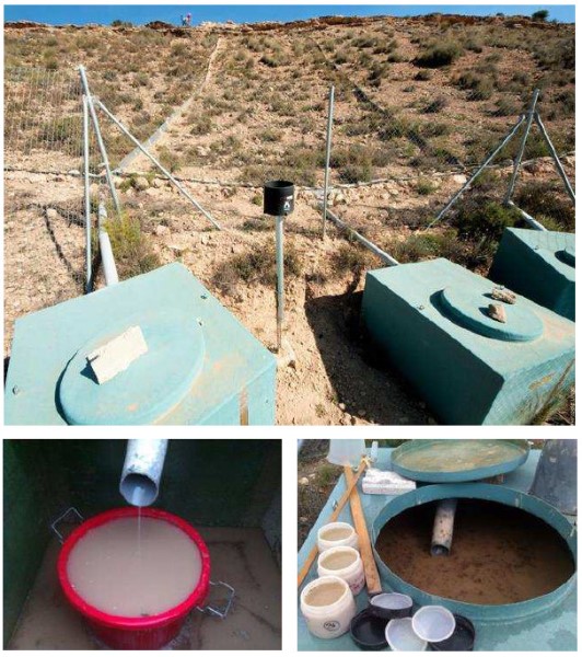
Sediment and runoff monitoring
To assess the effect of the vegetation-removal treatment on the redistribution of water by runoff within the experimental plots, we installed TDR (Topp and Davis 1985) soil-moisture probes (0-15 cm depth) upslope of nine vegetation patches (Lygeum tussocks) per plot. These patches varied in the size of the bare-soil interpatch upslope each of them, with patches in plot IC15 having the largest upslope bare-soil interpatches, and patches in plot IC45 having the smallest ones. For selected well-forecasted large rainfall events, we measured soil water content (SWC) the day just before the event and the day after, estimating from the difference in soil moisture between these two days the water gains for each vegetation patch.
Differences in runoff and sediment yield between the experimental plots (treatment effect) were analysed by ANCOVA, using rainfall amount or rainfall intensity (I15) as covariable. The relationships between the size of the upslope interpatch area and the water input gained after a rainfall event were analysed by regression analysis. These analyses and all statistical analyses described hereafter were performed using R (R Core Team, 2013).
Microtopography and erosion potential
Starting in May 2014, we monitored the profile dynamics of main rills developed on the experimental plots after the vegetation-removal treatment. We identified in the field and marked the most conspicuous rills developed on each plot. We then installed a number of regularly spaced pairs of fixed rods transversal to the main axis of each rill. Periodically, we assessed the variation in the profile of the rills by using a simple two-dimensional microprofilemeter mounted on these pairs of rods.
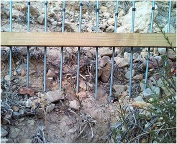
Microprofile meter
On May 15, 2015, using a Remote Piloted Aircraft (RPA) equipped with a GPS system, we took 203 aerial images of the experimental area. From these images, we generated a high resolution orthophoto (5.7 mm per pixel) and a DEM (11.5 mm per pixel) of the area. Further treatment of the images we performed with QGIS and GRASS software. Using the high resolution DEM, we estimated a modified LS factor of RUSLE (Renard et al. 1997) for each pixel in a raster map with a resolution of 5 mm per pixel. The S-factor measures the effect of slope steepness, and the L-factor defines the impact of slope length. The combined LS-factor describes the effect of topography on soil erosion. Values of LS factor are dimensionless and represent relative values compared to soil loss from a field under the standard conditions of 22.1 m length and 9 percent steepness. Our calculation of the modified slope length (LS) factor was based on slope and (specific) catchment area, the latter as substitute for slope length (see, for example, Panagos et al. 2015). We used one of the hydrology modules (Module LS factor) available in SAGA (System for Automated Geoscientific Analyses) software, which provides numerous applications for data analyses focusing on DEMs. This module takes a Digital Elevation Model (DEM) as input and derives catchment areas according to Freeman (1991). Using this module we generated maps for each plot representing the modified LS for each pixel, so that larger values indicate higher erosion potential. Rills concentrate runoff from microcatchments and have local high slope angles; thereby they typically yield high LS values, which helps to easily identify them on a LS map.
Soil surface condition and functioning
We assessed soil surface condition and functioning following the LFA methodology (Tongway and Hindley, 2004). We estimated the LFA soil functional indices (stability, infiltration and nutrient cycling indices), by combining field measurements of eleven soil features (Table). Using 50 cm × 50 cm sampling quadrats, and following a rating scale (Tongway and Hindley, 2004), these soil features were measured for the four types of bare-soil microsites: upslope, lateral and downslope a patch of Lygeum spartium, and isolated bare-soil interpatch. Ten sampling cuadrats were assessed per type of microsite and plot in March and October 2013, September 2014 and July 2015.
Table: LFA functional indices and soil surface features used to estimate each of them (Tongway and Hindley 2004).
| LFA index | Soil surface features considered |
| Stability index (%) | Ground cover; litter cover, crust cover; crust fragmentation; erosion type and severity; amount of deposited materials; surface resistance to disturbance; and crust stability. |
| Infiltration index (%) | Canopy cover; litter cover; soil surface roughness; crust stability; and soil texture |
| Nutrient cycling index (%) | Canopy cover; litter cover, origin, and degree of decomposition; crust cover; and soil surface roughness |
Vegetation performance, pattern, and dynamics
Plant cover was monitored by the point intercept method along three (25-m length) permanent transects per plot (125 points per transect). Plant cover and species number were recorded in November 2012, June 2013, August 2014, June 2015, and April 2016.
From the orthophoto obtained with the RPA on May 2015, we created a binary map and estimated total plant cover on each plot. Combining the orthophoto and the DEM, we calculated the index Flowlength (FL) for each plot. Flowlength quantifies the connectivity of bare-soil areas considering both vegetation pattern and topography. It is calculated as the average of the runoff pathway lengths from all the cells in a raster-based map of the area (Mayor et al. 2008).
Finally, to improve our understanding of the role of source–sink dynamics in plant productivity in drylands, and gain insights on the local (patch-scale) effect of pattern-driven resource redistribution, we monitored 10 individual Lygeum tussocks per plot and estimated the tussock basal growth (change in basal diameter with time), and reproductive effort (number of spikes per tussock basal area unit). Since tussock growth may depend on the tussock size (in turn depending on age), we represented tussock growth relative to the initial size. We studied these relationships using regression analyses. We compared growth and reproductive effort between plot treatments using repeated measures ANOVA.
Note: For full references to papers quoted in this article see