| Authors: | Bautista S, Fornieles F, Urgeghe AM, Román JR, Turrión D, Ruiz M, Fuentes D. and Mayor AG |
| Editor: | Jane Brandt |
| Source document: | Bautista S et al. (2016) The role of increasing environmental pressure in triggering sudden shifts in ecosystem structure and function. CASCADE Project Deliverable 4.2 35 pp |
Inter-calibration of experimental plots
During the 2-years inter-calibration period, the hydrological response of the three experimental plots was very similar. There were no statistical differences between plots regarding the relationships between rainfall and runoff (Figure 1). Although we measured some between-plots differences in runoff production in response to small rainfall events, they were minor differences, probably related to differences in the runoff produced very close to the plot outlet. Conversely, the runoff produced by large rainfall events was almost identical in the three plots. We obtained similar results regarding sediment yield, as well as using other rainfall metrics, such as rainfall intensity (data not shown).
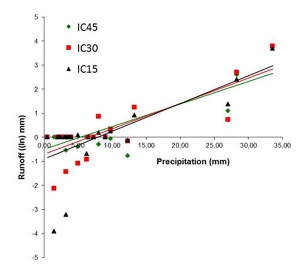
Figure 1
Given the lack of differences in the hydrological response of the three experimental plots, the differences found after treatment application were attributed to the treatment effect.
Hydrological response
During the study period reported here (Nov 2012-March 2016), we recorded 40 rainfall events that produced runoff on one or more plots (Figure 2). These events totalized 501 mm, 60% of total rainfall in the area in that period. The temporal variability of runoff-producing rainfall events was very high, with many medium-size events concentrated in autumn of 2012 and 2014, few very large events in spring 2013 and autumn 2015, and long dry intervals between these periods. It is worth noting the extraordinary dry period occurred between July 2013 and October 2014, only interrupted by six events that produced runoff. The year 2015 was also extremely dry, with only five events that produced runoff, yet one of them was particularly large.
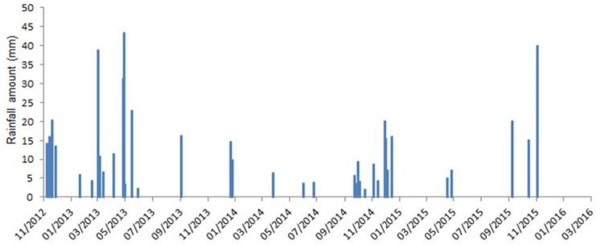
Figure 2
Total runoff produced over the study period was 3.7 mm, 11.1 mm. and 13.2 mm, for plots IC45, IC30, and IC15, respectively, which means that 0,4% to 1,6% of total rainfall was lost as runoff from the experimental plots. At the event scale, runoff coefficients for runoff-producing events ranged between 0.01% and 4.22% (average 0.33%) for IC45; 0.33%); 0.01% and 13.94% (average 0.99%) for IC30; and 0.01% and 9.20% (average 1.30%) for IC15. Most of this runoff was produced during the first six months of the experiment, before the severe 2013-2014 drought, while the longer but drier period of July 2013-March 2016 yielded approximately half of the runoff produced over the first six months (Figure 3). The production of sediment yield followed the same pattern, In general, plots IC30 and IC15 produced much higher runoff and, particularly, sediments than IC45, with IC15 showing only slightly higher yields than IC30 (Figure 3).
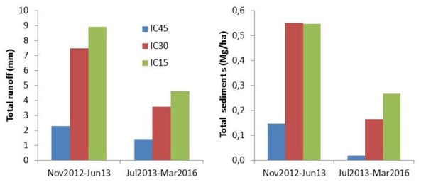
Figure 3
Rainfall-runoff and rainfall-sediments relationships and ANCOVA analysis (Figures 4 and 5; Table 1) showed significant variation in the hydrological and erosional response of the three plots (i.e., significantly different regression slopes, as expressed by significant interaction effect treatment x rainfall; Table 1), with almost identical response to rainfall of plots IC30 and IC15, and much higher production of runoff and sediments in these two plots than in IC45 for any given rainfall intensity higher than ∼20 mm h-1. The best explanatory rainfall variable was the AI15 index, which captures the influence of both rainfall amount and intensity (Figure 4). Results for only rainfall amount or intensity were similar, yet rainfall amount explained less of the variation in runoff and sediment yield (Figure 5; note R2) and showed weaker treatment and rainfall-treatment interaction effects than AI15 (Table 1).
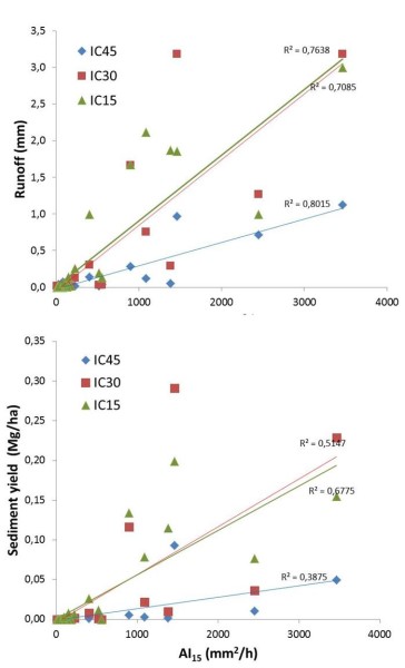
Figure 4 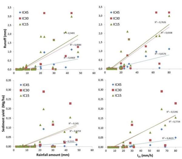
Figure 5
Table 1. ANCOVA results (F and p values) for treatment and rainfall (covariable) main effects and interaction effect on runoff and sediment yield. Treatments: IC45, IC30, IC15. Covariables: maximum rainfall intensity in 15 minutes (I15; mm h-1), rainfall amount (A, mm), and AI15 index (mm² h-1)
| Effects | Runoff | Sediments | ||
| F | P | F | P | |
| I15 Treatment I15 * Treatment |
230.2 1.6 19.2 |
˂ 0.001 0.201 ˂ 0.001 |
155.9 1.8 16.8 |
˂ 0.001 0.168 ˂ 0.001 |
| Rainfall amount (A) Treatment A * Treatment |
86.8 0.83 7.3 |
˂ 0.001 0.44 0.001 |
40.6 0.62 5.2 |
˂ 0.001 0.538 0.007 |
| AI15 Treatment AI15 * Treatment |
280.1 0.28 21.0 |
˂ 0.001 0.755 ˂ 0.001 |
123.6 0.15 13.9 |
˂ 0.001 0.861 ˂ 0.001 |
The residuals from the relationships shown above between rainfall and runoff or sediment yield (using the best explanatory variable: Maximum intensity in 15 minutes, I15) can be plotted against time since treatment implementation. This type of graphical representation (Figure 6) provides information on the trends in the hydrological behaviour once the effect of the magnitude and/or intensity of the rainfall have been removed from the analysis. For the three experimental plots, the residuals from the regression between runoff and AI15 index showed a constant trend, which indicates that the capacity of the plots for producing runoff (i.e. losing resources) did not significantly vary with time since treatment application. This means that, for any given type (amount-intensity) of rainfall, the hydrological response of the plots was more or less the same either soon or long time after treatment application.
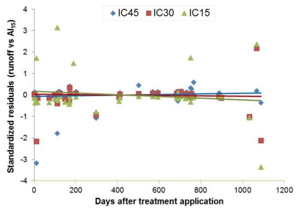
Figure 6
The relationships between sediment yield and runoff were very similar for all plots (Figure 7, left), with IC30 showing a higher slope and therefore indicating a higher average sediment concentration in runoff than the other two plots. The residuals from these relationships plotted against the time elapsed since treatment application showed that sediment concentration in runoff did not vary with time, except for a hardly perceptible decreasing trend in IC15 (Figure 7, right).
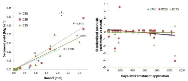
Figure 7
Regarding water redistribution at the patch scale, soil water gain upslope Lygeum tussocks after a runoff-producing rainfall event, varied between plots (F= 3,76; p=0,037; ANOVA), with higher water gains upslope tussocks in CI15 and lower in CI45 (Figure 8, left). The variation in soil water gains depended on the size (length) of the upslope interpatch (Figure 8, right).
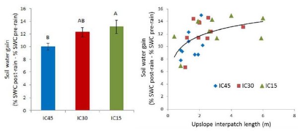
Figure 8
Microtopography
The assessment of rill-profile dynamics showed that the largest rills developed on plot IC15 (Figure 9), yet the average maximum depth for the assessment period was similar for rills on plots IC30 (5.1 ± 0.6 cm) and IC15 (5.0 ± 0.4 cm) and smaller for rills on IC45 (4.2 ± 0.4 cm). However, while rills on IC45 hardly varied their profile with time, rills on IC30 and IC15 showed a further increase in rill incision from May 14 to Sep 14 (Figure 9) followed by a partial refilling of the rill (from Sep 14 to Dec 14).
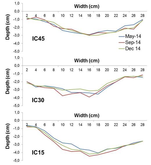
Figure 9 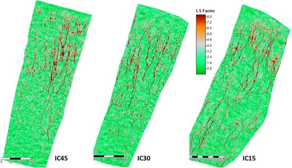
Figure 10
From the high resolution orthophoto taken in May 2015, we estimated the spatial variation and average value per plot of the LS factor, which captures the contribution of topography to erosion potential. Average LS-factor values were 2.23, 2.77, and 2.75, for IC45, IC30 and IC15, respectively. The spatial variation of LS factor highlighted the rill network of each plot, which showed longer and denser rills in IC30 and IC15 plots than in IC45 (Figure 10). While IC45 concentrated high LS values and a rill area on the top of the plot that did not connect with the plot outlet, IC30 and, particularly, IC15 showed highly connected network of rills and high LS areas.
Soil surface condition and functioning
In general, bare-soil interpatch areas (microsites) located next to a vegetation patch (e.g. lateral interpatch) showed slightly higher values for the LFA soil functional indices than interpatch areas located at certain distance from vegetation patches (isolated interpatch), particularly for the Infiltration and Nutrient cycling indices (Figure 11).
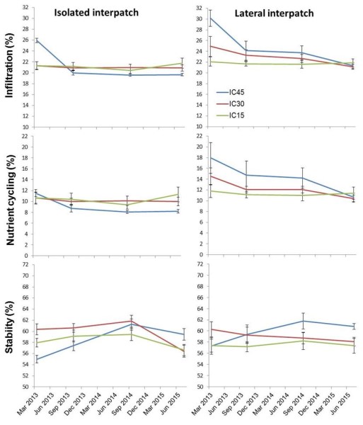
Figure 11
Isolated bare-soil interpatches on plots IC30 and IC15 showed no variation with time for the Infiltration and Nutrient cycling indices, whereas IC45 showed higher values for these two indices at the beginning of the monitoring period (March 2013) that rapidly decreased and then stabilized at slightly lower vales than IC30 and IC15 (Figure 11). Conversely, the stability index for isolated interpatches showed an increasing trend during the first 1.5 year of the monitoring period (March 13 - Oct 14), particularly for IC45 plot, which changed from initial (March 2013) lower values to final (June 1015) higher values than IC30 and IC15.
Bare-soil interpatch areas located next to vegetation patches (lateral interpatches) showed a very similar pattern for Infiltration and Nutrient cycling indices: lower values and no variation with time for IC15; a clear decreasing trend for IC45; and a slight decreasing trend for IC30, which all together resulted in no differences between plots at the end of the monitoring period (Figure 11). The Stability index for lateral interpatches showed no variation or slight decreasing trend for IC15 and IC30, respectively. However, IC45 showed an increasing trend with time, which resulted in higher values of this index for IC45 than for the other two plots at the end of the monitoring period.
Likewise lateral interpatch areas, interpatch areas located upslope or downslope a vegetation patch also showed higher values than isolated interpatch areas. However, these two types of interpatch area showed less variation with time and between experimental plots (data not shown).
Vegetation performance and dynamics
The dynamics of plant cover and number of species reflected the impact of both the plant-removal treatment and the severe 2013-14 drought (Figure 12). During the first rainy period and growing season after the treatment application, plant cover increased in all plots. Then, in response to the drought, plant cover decreased in all plots, particularly in IC30. After the drought, plant cover stabilized around 20-25% cover in IC15 and IC30 plots, and slowed down the decreasing trend in IC45. Only during the last year of the monitoring period reported here, plant cover has showed certain degree of recovery, resulting in value around 30% for IC15 and IC30 plots, and close to 40% for IC45 plot (Figure 12, left), still very far from the original pre-treatment values. The number of species followed a similar dynamics (Figure 12, right).
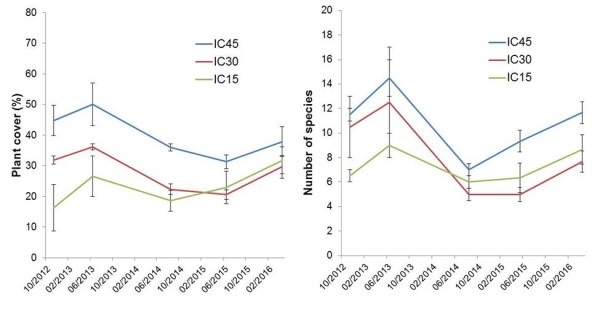
Figure 12 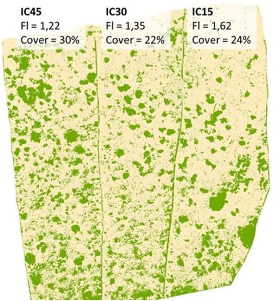
Figure 13
In May 2015, total plant cover values estimated from a high-resolution aerial picture taken from a Remote Piloted Aircraft (Figure 13) fully matched the values estimated from the field transects for that period. The between plot variation in bare-soil connectivity (estimated by the Flowlength index; Mayor et al. 2008), did not match the variation in plant cover, as IC15 showed higher bare-soil connectivity than IC30 despite having a similar, slightly higher plant cover value. Average patch size for IC45, IC30 and IC15 were 292 ± 33 cm², 239± 22 cm², and 423± 85 cm², respectively.
The growth of Lygeum spartum tussocks (relative to their initial size) showed different trends between the different plots and the dates on which they were measured (Figure 12). During the first part of the assessment period (May 2013 - May 2014) individuals of IC15 and IC30 plots showed an increasing trend in growth with increasing initial size, while individuals of IC45 plot showed the opposite trend (Figure 14,left). During the second part of the assessment period (May 2014 - May 2015), the observed trends were almost opposite to the ones observed the previous period, so that individuals of plots IC30 and IC15 showed a decreasing trend in growth with increasing initial size, especially clear in individuals of IC30. Individuals of IC45 did not show any effect of the initial size on their growth during this period (Figure 14, right). However, these differences in trend between plots were not statistically significant (ANCOVA Analyses).
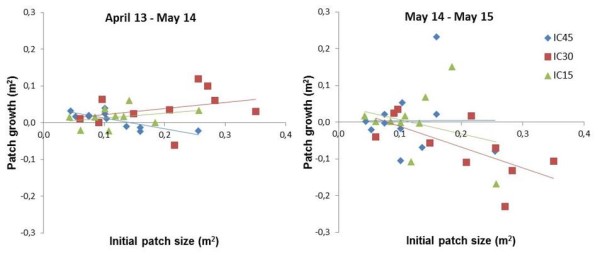
Figure 14 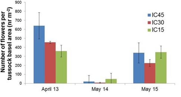
Figure 15
Production of flowers by Lygeum individuals showed a clear impact of the drought period, which reduced production to almost zero, but not did not show any significant effect of the treatment, except for a slight, non-significant decreasing trend from IC45 to IC15 during the first assessment period (Figure 15).
Note: For full references to papers quoted in this article see