| Authors: | Alejandro Valdecantos (CEAM),V. Ramón Vallejo (UB), Susana Bautista (UA), Matthijs Boeschoten (UU), Michalakis Christoforou (CUT), Ioannis N. Daliakopoulos (TUC), Oscar González-Pelayo (UAVR), Lorena Guixot (UA), J. Jacob Keizer (UAVR), Ioanna Panagea (TUC), Gianni Quaranta (UNIBAS), Rosana Salvia (UNIBAS), Víctor Santana (UAVR), Dimitris Tsaltas (CUT), Ioannis K. Tsanis (TUC) |
| Editor: | Jane Brandt |
| Source document: | Valdecantos, A. et al. (2016) Report on the restoration potential for preventing and reversing regime shifts. CASCADE Project Deliverable 5.2 104 pp |
- The degraded state represents an ‘old’ shrubland where gorse disappeared by natural senescence and was dominated by rosemary
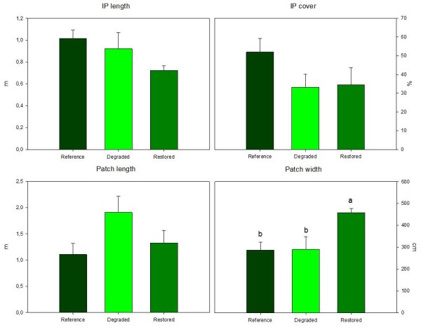
- The bigger size of patches in the restored areas can be related to the collapse of old shrubs in the degraded plots resulting in openings in the continuous shrubland
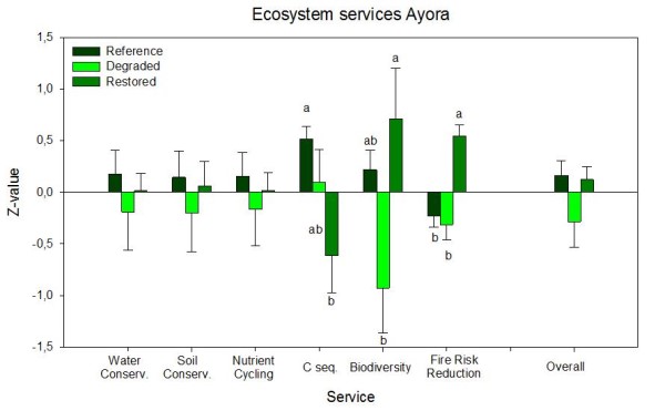
- Biodiversity was the most improved service by restoration actions
- But also the restoration approach considered in Ayora, with the reduction of levels of understory biomass, improves the ecosystem service ‘fire risk reduction’ even ten years after the application of treatments
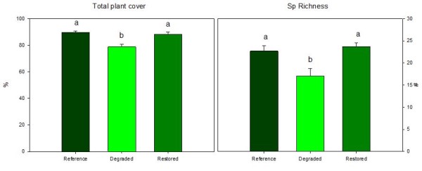
Plant cover in Ayora ecosystems ranged between 78.8 and 89.6% with significant differences between the degraded and the other two systems (Figure 1 left). We found fifty-two vascular plant species in the sites, eight of them (subshrubs except the shrub Rhamnus lycioides) were exclusively present in the reference forests. The average number of plant species in the restored and the reference sites were significantly higher than in the degraded plots (23.7, 22.7 and 17.0, respectively; Figure 1 right). Eleven species corresponding to both shrubs and subshrubs were only found in the restored plots, two of them (Pistacia lentiscus and Rhamnus alaternus) were introduced by planting. The reference communities correspond to pine forests of Pinus pinaster and P. halepensis (47.9 and 11.4% of cover, respectively) with two dominant species in the understory (Rosmarinus officinalis - 26.4% - and Ulex parviflorus - 13.3%) and scarce abundance of grasses (Brachypodium phoenicoides and B. retusum with 8.3 and 6.3%, respectively). The degraded shrublands are dominated by the shrubs R. officinalis (44.3%) and Erica multiflora (15.7%) and larger herbaceous layer (B. retusum and Helictotrichon filifolium, 21.3 and 10.8%, respectively). The species dominance inverted in the restored plots, with B. retusum being the most abundant species (40.2%) and R. officinalis dominating the shrub layer (26.2%). Other species with cover percentages above 10% were the shrub U. parviflorus (12.7%) and the grasses B. phoenicoides (12.5%) and Stipa offneri (10.7%).
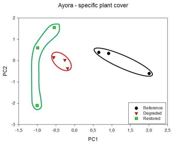
The two first axes of the principal component analysis accounted for 43.1% of the total variance and plots were clearly separated, especially, along the first component (Figure 2). The reference plots showed the highest positive scores of PC1, the restored plots released the most negative ones while the degraded showed intermediate values but closer to the restored than to the reference sites. We also observed high variability in species composition and contribution within the three spatially replicates restored plots as showed by wide range of values along the second axis. Degraded areas were plotted in a tight group according with these two axes.
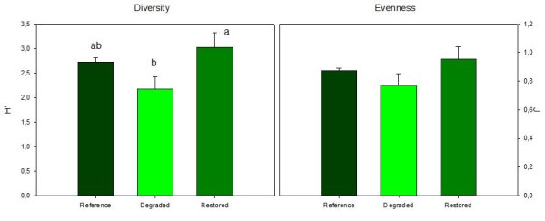
Diversity indexes, especially Shannon-Wiener’s, were also affected by restoration (Figure 3). The H’ value was significantly higher in the restored plots (3.0) than in the degraded (2.2) with the reference areas showing intermediate values. Evenness values were quite similar but in this case differences were not statistically significant.
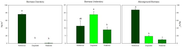
Biomass accumulation in the different layers of the ecosystem was also dependent of the ecosystem state (Figure 4). Obviously, the biomass in the overstory was extremely higher in the reference than in the other two states where pine recovery was almost null. Regarding the understory (both shrubs and grasses), the degraded plots showed higher biomass than the restored areas. In fact, understory biomass in untreated degraded shrublands were two-fold that in the cleared plots. As a consequence, and because the contribution of the overstory in these two types of shrublands is negligible, the total aboveground biomass accumulated in the degraded was significantly higher than in the restored plots.
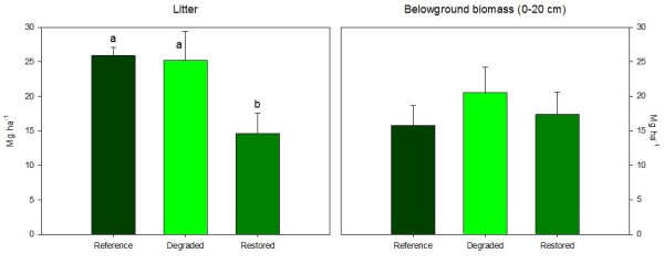
The litter layer in both the reference and the degraded areas were very similar although the origin of the plant material was quite different (mostly pine needles in the reference and fine and coarse shrub debris in the degraded). The restored plots showed significant reductions, above 40%, of litter accumulation (Figure 5 left). Root biomass in the most superficial 20 cm of soil did not show significant changes due to the state of the ecosystem and ranged between a minimum of 15.8 Mg ha-1 in the reference to a maximum of 20.6 Mg ha-1 in the degraded plots (Figure 5 right).
In relation to the distribution and morphology of the sink and source areas within the landscape, the considered interpatches in Ayora included bare soil but also the matrix of perennial grasses and litter, very abundant in the three ecosystem states as it has already been mentioned. The length and percentage of interpatches in the forest systems were slightly higher than in the two shrubland systems. Interpatches averaged 1.0, 0.9 and 0.7 m in the reference, the degraded and the restored plots, while their cover was 52% in the forest and 33-34% in the two shrubland types (Figure 6). The size of patches was increased by restoration with an average width of 4.6 m while both in the reference and in the degraded plots patches were 2.9 m wide.
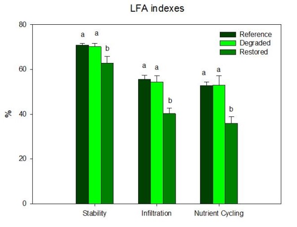
The three indexes derived from the LFA assessment showed a significant reduction in the restored system while no differences were observed between the reference and the degraded states (Figure 7). The more pronounced reduction was observed in the nutrient cycling that fell from 53% to 36% in the restored plots. Also the infiltration was sharply reduced, with values around 55% in the reference and degraded sites and 40% in the restored. The reduction in the stability index was slightly lower but however differences between states were also significant.
Half of the ecosystem services were significantly affected by the state of the ecosystem: C sequestration, biodiversity and fire risk reduction (Figure 8). The other three services (soil and water conservation and nutrient cycling), and the combination of all of them as well, showed the same trend to decrease from the reference to the degraded state while the restored showed intermediate values. The fire and the extremely limited post-fire recovery of pines, combined with the selective clearing of flammable shrubs, resulted in a significant reduction of C sequestration in the restored plots. On the contrary, restoration improved biodiversity of the degraded shrublands even beyond values of the reference state of the ecosystem. The most significant effect of the restoration actions was in reducing fire risk in relation to both the reference and the degraded plots. This was the main objective pursued with the restoration conducted in the degraded areas ten years before this assessment.
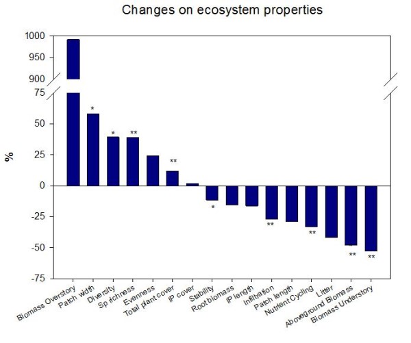
The summary of changes of ecosystem properties due to restoration (Figure 9) showed postive effects on variables related to community composition and structure (diversity indexes and patch-interpatch distribution and morphology) while negative chenges were mainly associated to biomass accumulation (litter, understory and nutrient cycling and infiltration). However, large amounts of biomass in the understory in the degraded areas increases the C sequestred in the system but also increases flammability and, hence, fire risk.
Note: For full references to papers quoted in this article see