| Authors: | Alejandro Valdecantos and Ramón Vallejo (CEAM) with input from study sites |
| Editor: | Jane Brandt |
| Source document: | Valdecantos & Vallejo. (2015) Report on structural and functional changes associated to regime shifts in Mediterranean dryland ecosystems. CASCADE Project Deliverable 5.1. |
A common methodology was applied in all six CASCADE field sites to assess Ecosystem Services in, at least, two ecosystems representative of a healthy reference and a degraded state. However, the protocol has been adapted locally to fit singularities, constraints and possibilities of the different field sites. The general framework includes the identification of representative Reference and Degraded ecosystems according to the pressure acting in each specific site.
Table: Summary of pressures, reference and degraded ecosystems in the six CASCADE field sites
| Field Site | Pressure | Reference Ecosystem | Degraded Ecosystem |
| Várzea, PT | Fire | Pinus pinaster forest | 4-times burned areas (2-years after last fire) |
| Albatera, SP | Multifactor (climate, historical use and mismanagement) | Semi-steppe dry shrubland | Dwarf shrubland |
| Ayora, SP | Fire | Unburned Pinus pinaster and P. halepensis forest | Shrubland. Areas burned in 1979 |
| Castelsaraceno, IT | Grazing | Productive pastureland | 1.Overgrazed lands 2. Undergrazed lands |
| Randi, CY | Grazing | Shrubland | Unpalatable community |
| Messara, GR | Grazing | Shrubland | Unpalatable community |
Three spatially replicated plots were established for every level of pressure in every field site to conduct the assessment of different variables of ecosystem structure and functioning. Replicated plots shared most physiographic, climatic, and edaphic variables as well as land use history. From these variables, we calculated a balanced set of ecosystem services. The effects of degradation on the ecosystem structure and function as well as on ecosystem services were derived through a comparison of the Reference with the Degraded state.
The following were measured and calculated:
- determination of plant composition,
- quantification of stand plant biomass,
- quantification of litter and belowground biomass, and
- application of the methodology of Landscape and Function Analysis.
1. Plant composition
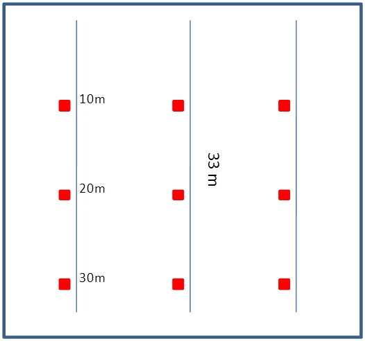
Three 33m linear transects (as straight as possible) were deployed following the maximum slope and the line intercept method was applied. A metal rod (<5 mm diameter) was placed vertically every 50 cm along the tape (66 points per transect) and the contacts of plant species recorded. The contact at the soil level was also described (bare soil, stone, rock outcrop, litter, biological crust). Several plants may touch the rod in a particular point and all of them were recorded as well as the height where the plant contacts the rod. Note that this allows plant cover percentages above 100% due to overlapping.
Transects were deployed avoiding ‘strange’ or artificial features of the plot such as pathways, stone accumulation points, gullies. In case that the size of the plot did not allow 33-m long transects, more shorter transects were established but always totalling 100 m per plot.
2. Plant biomass
Three 1-m² quadrats (subplots) were defined in every transect. The placement of the quadrats was predefined to avoid subjective selection of microsites. For instance and in the case of a 33 m transect, we placed the subplots at 10-11 m, 20-21 m and 30-31 m (one meter away from the tape). Within these subplots we evaluated biomass of shrubs by two alternative approaches:
- By clipping, drying and weighing. When possible, we cut all the individuals whose stems were within the quadrat limits and took them separately (one bag per species and subplot) to the lab. We dried the plant samples at 60ºC for 48h in an oven and weighed them. Grasses were not separated by species.
- By allometric relations. There are available allometric equations for many of the most common shrub species in the Mediterranean Basin. By knowing a morphological variable (basal diameter, total height or biovolume of the plant), we calculated the biomass of the individuals. Alternatively, as was the case of some shrub species in Messara and Randi field sites, we built up our own allometric equations by harvesting, drying and weighing a pool of individuals outside the plots covering the range of plant sizes present within the plot.
3. Litter and belowground biomass
After harvesting grasses and shrubs, we collected the litter layer in a 25 x 25 cm sub-subplot. We avoided taking mineral soil particles in the samples as they are much heavier than the litter fractions. Samples were taken to the lab to dry them at 60ºC for 48h. In the same sub-subplot once the organic layer was removed we took a soil core of the uppermost soil (0-10, 0-15 or 0-20 cm depending on the site). Once in the lab, roots were separated from the soil by sieving and washing gently with water before drying at 60ºC for 48h.
4. Landscape and Functional Analysis (LFA)
The following is a highly synthesised description of the method used for the assessment of ecosystem functioning.
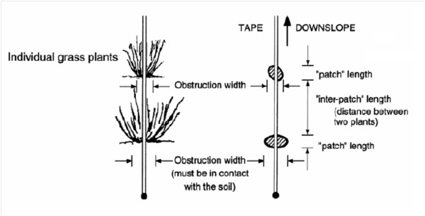
- Transects set-up: Transects started at the downslope edge of a patch following the maximum slope and as taut as possible.
- Patch and inter-patch identification: By definition, patch accumulates or diverts resources by restricting flow of water, topsoil and organic matter (e.g. perennial plants , stones > 10 cm). They act as a sink of resources. But not all patches behave the same and we discriminated when possible between different patches, e.g. resprouter shrub, seeder shrub, grasses, chamaephytes. Inter-patches represent areas where resources do not accumulate and even act as net export of resources (source areas). We measured three parameters along the transects: the number of patches (sinks), the width of every single patch (at the soil level, not the canopy and up to a maximum of 10 m), and the distance between patches (inter-patch length). However, in some field sites (e.g. Ayora) the continuity of vegetation hindered clear measurements of patch characteristics.
- Soil Surface Assessment: This assessment was conducted per plot in five 50 x 50 cm areas per type of identified patch and inter-patch. These five replications were distributed throughout the plot. The soil surface assessment is rapidly made by the use of simple visual indicators. These indicators are:
• Rainsplash protection: ephemeral grasses, foliage at heights above 50 cm and litter were excluded.
• Perennial vegetation cover
• Litter: amount, origin and degree of decomposition. It includes annual grasses and ephemeral herbage (both standing and detached) as well as detached leaves, stems, twigs, fruit, dung, etc. There are three properties of litter that were assessed in the following order: Cover (% and thickness of the litter layer), Origin (whether it is local or transported) and Degree of Decomposition/Incorporation.
• Cryptogam cover
• Crust brokenness
• Soil erosion type and severity: Five major forms of erosion were assessed: Sheet erosion (progressive removal of very thin layers of soil across extensive areas, with few if any sharp discontinuities to demarcate them), Pedestal (is the result of removing soil by erosion of an area to a depth of at least several cm, leaving the butts of surviving plants on a column of soil above the new general level of the landscape), Terracette (abrupt walls from 1 to 10 cm or so high, aligned with the local contour), Rill (channels cut by the flowing water), and Scalding (is the result of massive loss of A-horizon material in texture-contrast soils which exposes the A2 or B horizon).
• Deposited materials: presence of soil or litter materials transported from upslope.
• Soil surface roughness: due to soil surface micro-topography or to high grass density.
• Surface nature: resistance to disturbance.
• Slake test: The test was performed by gently immersing air-dry soil fragments of about 1-cm cube size in distilled water and observing the response over a period of a minute or so. If the soil floats in water (high organic matter), then it is stable (Class 4), and if it cannot be picked (loose soils) was scored as not applicable.
• Texture
Spreadsheets were prepared and were filled out with the collected information and Stability, Infiltration and Nutrient Cycling indices were automatically calculated. These indices varied between 0 and 100% depending on ecosystem functionality (100% represents fully functional systems).
Table: List of the soil functional indicators and their contribution to the indices of stability, infiltration and nutrient cycling (following Tongway and Hindley 2004). x means that the indicator is scored in the calculation of the index given above.
| Indicator | Indices | ||
| Stability | Infiltration | Nutrient Cycling | |
| Rainsplash protection | x | ||
| Perennial vegetation cover | x | x | |
| Litter cover | x | x | |
| Litter origin and decomposition | x | ||
| Cryptogam cover | x | x | |
| Crust brokenness | x | ||
| Soil erosion type and severity | x | ||
| Deposited materials | x | ||
| Soil surface roughness | x | x | |
| Surface nature | x | x | |
| Slake test | x | x | |
5. Data analysis
In every CASCADE field site we conducted t-test (sites with one Reference and one Degraded state of the ecosystem) or one-way ANOVA followed by post-hoc analysis (where three ecosystem states were identified) to assess if observed differences in all composition, functional, diversity and service variables were statistically significant. We conducted Principal Component Analysis (PCA) on specific plant cover data to assess general changes in vegetation composition and cover between Degraded and Reference sites.
Table: List of ecosystem services measured, variables from which their relative states were estimated through standardization,
and the methodology used to obtain the data of the variables.
| Ecosystem Service | Variables | Methodology |
| Water Conservation | Infiltration Index Interpatch Cover Plant Cover |
LFA + Point-intersect |
| Soil Conservation | Stability Index Interpatch Cover Plant Cover |
LFA + Point-intersect |
| Nutrient Cycling | Nutrient Index Litter |
LFA |
| Carbon Sequestration | Plant biomass Root biomass Litter |
Allometries + direct quantification |
| Biodiversity | Richness Diversity Evenness |
Point-intersect |
Acquired data of structural and functional ecosystem properties were then grouped into related ecosystem services through standardization. We have selected regulating and supporting services as well as biodiversity, which underpins all services. Each variable was standardized using
ZPlot = (XPlot - AvgTot) / SDTot
where ZPlot is the standardized variable, XPlot the original variable, AvgTot the average of the variable of all plots within a field site and SDTot the standard deviation of all the plots within a field site. Variables were assigned to services as they were derived from validated methodologies selected on the basis of being appropriate indicators for this service. When several variables were combined into one service, each variable was weighted equally, as all of them are considered to be good indicators for the respective service and no available information points to a better performance of any of them. The five selected ecosystem services were also weighted equally and averaged for Degraded and Reference plots in each field site as a global result of ecosystem service losses. This way, the assessment provides a baseline integrated and global evaluation based on the simplest assumption. However, it is worth mentioning that stakeholders’ preferences regarding ecosystem services could be incorporated in the assessment in the form of different weights for each service, which could yield different global outcomes.
Note: The selection of the key common indicators and assessment methods has been based on the work developed by the EU-funded PRACTICE project on ground-based assessment indicators. They represent few essential indicators that could characterize ecosystem function for a majority of drylands worldwide, mostly focusing on water and soil conservation, nutrient cycling, carbon sequestration, and biological diversity. Most provisioning and cultural services are considered to be very much context dependent. Furthermore, half of the sites included in CASCADE are natural areas that are not expected to directly deliver goods. Therefore, our across-site comparative assessment of ecosystem services provision has been only based on supporting-regulating services, which together with biodiversity, are considered to be baseline services and properties that underpin other types of services.
References
For ease of reading, references to other scientific work have been removed from this page. See the full report for details of all the citations