| Main authors: | Diana Sietz, Luuk Fleskens, Lindsay C. Stringer |
| Editor: | Jane Brandt |
| Source document: | Sietz, D. et al. (2017) Report on integrated modelling strategy. CASCADE Project Deliverable 8.2 33 pp |
Guiding land management through a perspective on non-linear ecosystem dynamics
Widespread failure in ecosystem restoration and degradation prevention, even with massive investments, has underpinned the broad agreement that ecosystems can behave in complex, non-linear ways (Westoby et al. 1989, Scheffer et al. 2001). In contrast to gradual responses, several studies demonstrate that a range of terrestrial and aquatic ecosystems exhibit alternative dynamic regimes and threshold dynamics (Scheffer and Carpenter 2003, Folke et al. 2004, Hirota et al. 2011, Suding 2011). Restoration of ecosystem performance after a decline and prevention of degradation can require considerably stronger efforts in non-linear than in gradually responding systems, but can also benefit from particular opportunities due to non-linear dynamics. Hence, recognition of dynamic ecosystem regimes and threshold dynamics can provide crucial advances to operationalising LDN.
A dynamic ecosystem regime is a region in a state space – also called a basin of attraction – in which an ecosystem develops towards a stable equilibrium (Scheffer et al. 2001). Small disturbances or management impacts can change an ecosystem’s state, but the system remains within a given regime and ultimately tends towards the stable equilibrium due to positive internal feedbacks. Dynamic regimes are separated by thresholds defined as boundaries in time and space. At a threshold, a small change in environmental conditions, such as precipitation variability, herbivore pressure, fire frequency or soil fertility, triggers a large change in ecosystem state implying abrupt shifts from one dynamic regime to another. Existence of two alternative dynamic regimes under the same environmental conditions implies hysteresis (Figure 1a) such that a system’s degradation path can strongly differ from its restoration path. Severe disturbances or large management impacts can shift the system over the border of a basin of attraction to an alternative basin of attraction. Changes in environmental conditions exceeding a threshold (T1 and T2 in Figure 1a) can also trigger a regime shift. Responses manifest as alterations in the productivity and cover of grasses, shrubs or trees and species composition as well as other ecosystem state variables. Such alterations can demand minor or major investments in order that they may be avoided, reduced and/or reversed.
A grass- and a shrub-dominated landscape can be considered as two alternative regimes, which are useful to illustrate shifts in internal feedbacks. Intense livestock grazing can drive degradation shifts from grassland (healthy state) to shrubland (degraded state), leading to decreased fuel connectivity and lack of fire disturbance (Friedel 1991). Without fire, germinating shrubs which are not grazed can survive and outcompete grasses. Under significantly changed feedback mechanisms governed by grass-shrub competition, shrubs can persist even after grazing pressure reductions. Land management needs to reduce grazing intensity in order to improve environmental conditions well beyond the pre-degradation threshold at which the ecosystem shifted to the alternative regime (T2 in Figure 1a) for the grass-dominated regime to recover. This demonstrates that under hysteresis, ecosystem restoration may require greater efforts and investments compared with a non-hysteretic ecosystem. Changes in environmental conditions may alter regime boundaries and hence the size of a basin of attraction affecting its resilience to disturbance. An increase in basin size can reduce the probability of a regime shift, as the system is less easily driven over a threshold into an alternative regime, implying greater resilience. Likewise, preventive actions such as livestock rotation to reduce grazing pressure are crucial when a healthy grassland approaches a threshold (T2 in Figure 1a). By increasing the distance to a threshold, this can reduce the likelihood of a shift to the degraded shrub-dominated regime.
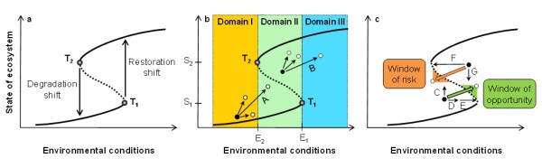
Figure 1
As ecosystems are complex systems displaying high variability in constituting processes and states, there is no single one-dimensional threshold that determines restoration or degradation outcomes. Underlying processes must therefore be adequately captured in threshold models to avoid misinterpretation of conditions under which ecosystems may not be restorable because a historical reference cannot be re-established (Bestelmeyer 2006). Recent work on ‘novel ecosystems’ highlights the necessity of distinguishing situations in which original states cannot be restored, for example due to constraining interactions between climate change and land use (Hobbs et al. 2013). Land management considering diverse ecosystem functions and multi-dimensional thresholds is a pre-requisite to achieve LDN.
An ecosystem’s state relative to critical thresholds can provide key insights into appropriate timings and urgency of restorative and preventive interventions. Ecosystems in a bi-stable situation (Domain II in Figure 1b) must be prioritised. Experimental evidence shows that arid grasslands in the southwestern United States that degraded to shrub-dominated ecosystems due to intensive grazing can be restored when livestock are excluded (Valone et al. 2002). In the dynamic regime perspective, livestock exclosure induced improved environmental conditions, up to or beyond E1 (see Figure 1b), enabling a restoration shift. However, shrub-dominated systems may respond slowly to livestock removal as a single management strategy, requiring >20 years before natural grasslands regenerate (Valone et al. 2002). These time lags create delays before management effects materialise highlighting that restoration efforts often require a long-term vision and commitment to be successful.
In a domain with a single degraded regime, Domain I in Figure 1b, land management principally cannot induce a shift to the healthy (e.g. vegetated) regime due to the absence of an alternative regime. Yet, management such as reduction in grazing pressure and erosion control (especially in regions with erodible soils, highly variable and intensive rainfall and strong winds) is required to avoid a further deterioration of ecosystem state, which would make restoration more difficult. For example, bush encroachment and repeated wildfires affecting abandoned landscapes are known to lead to long-term loss of productivity (Roques et al. 2001, Hill et al. 2008) and the high cost of reversing such degradation is prohibitive (Reed et al. 2015). Similarly, an ecosystem in Domain III cannot shift to an alternative regime, even with a severe disturbance. Here, land management would ideally maintain environmental conditions beyond E1 (Figure 1b), avoiding the possibility of a regime shift.
Identifying climate-dependent windows of opportunities and risks
Environmental conditions can strongly vary, opening windows of opportunities and risks for restoration and degradation prevention. Opportunities include exceptionally wet episodes, such as those associated with the El Niño Southern Oscillation (ENSO; Holmgren and Scheffer 2001). Field monitoring and remotely-sensed estimates of tree cover demonstrate that seeding (arrow C in Figure 1c) and protecting seedlings from herbivores (arrow D in Figure 1c) at the onset of a rainy El Niño episode (arrow E in Figure 1c) facilitated tree recruitment and regeneration of extensive dry forests in coastal Peru (Sitters et al. 2012). This fine-tuned dual management strategy was particularly successful in wetter low-lying areas and sandy soils. In contrast to seeding as a single restoration strategy, which was insufficient to induce forest restoration (Sitters et al. 2012), this combination can trigger the passage of thresholds, inducing sudden, long-lasting restoration shifts towards a high vegetation cover regime (green arrow in Figure 1c). These dual management strategies together with more frequent extreme precipitation events associated with future climate change may generate important windows of opportunities for the recovery of dry forests in some coastal regions in western South America (Holmgren et al. 2013) upon which people’s livelihoods rely. Benefitting from such opportunities however requires efficient flood and erosion control measures to avoid land degradation.
Land management to prevent degradation shifts must consider windows of risks when typical degradation drivers, such as drought and deforestation, interactively affect an ecosystem’s state. For example, dynamic modelling suggests that combined drought and deforestation can result in more widespread shifts from rainforest to savanna regimes in the south-eastern Amazon basin than those triggered by either drought or deforestation (orange arrow in Figure 1c; Staal et al. 2015). Here, both drought and deforestation favour grass invasion which increases flammability, decreasing the rainforest’s fire resilience and therefore increasing the probability of a degradation shift to a savanna regime. As the combined effects of drought and deforestation can move a forest out of Domain III into the bi-stable Domain II (see Figure 1b), land management is required to stabilise internal feedbacks (e.g. preventing fragmentation of forest canopy and grass invasion) in order to reduce the probability of a degradation shift. This underlines the importance of policies and mechanisms to prevent deforestation, particularly when future climate change is associated with more frequent and intense droughts (Malhi et al. 2008) and coupled degradation drivers limit the boundaries within which forests can be sustainably managed (Scheffer et al. 2015).
Deciding when to invest
For financial viability of investments, stability domains (Figure 1b) matter greatly, as does the opening of a climate-dependent window of opportunity or risk (Figure 1c). Cost-benefit analysis is traditionally applied to assess expected financial impacts of land management interventions (Qadir et al. 2014, Giger et al. 2015, Baptista et al. 2016). While the feasibility of interventions may depend on a variety of criteria, a major assumption is that a land manager would invest only in those measures whose expected returns are positive. It is however often difficult to anticipate the effects of land management with certainty (Suding 2011, Wilson et al. 2011, Nilsson et al. 2015).
A global meta-analysis of ecosystem restoration depicts large variations in benefit-cost ratios across a range of biomes including grasslands, forests and wetlands (De Groot et al. 2013). Similarly, a global analysis of successful SLM cases reveals great differences in the costs and benefits that stakeholders perceived in establishing and maintaining SLM measures depending on management type, region and area size (Giger et al. 2015). Further differentiation of costs and benefits according to varying degradation levels, environmental conditions and climate risks and opportunities is essential to inform investment decisions. Clearly, a better understanding of dynamic ecosystem regimes can advance decision making on investment in land management, particularly concerning large-scale restoration and SLM programmes. Here, timing is a key factor: investment costs are required immediately and maintenance costs may pose an additional strain on resources in the initial years following an investment, whereas the later the benefits are anticipated to occur, the less they are valued at the time of establishment of SLM programmes. In cost-benefit analysis this is captured through discounting of future costs and benefits. In the following paragraphs, we discuss the effects and cost-effectiveness of seeding as a key restoration measure to illustrate major differences in the costs and benefits arising from action across the stability domains. Seeding makes for a good illustrative case as it directly affects an ecosystem’s state and its success may vary with environmental conditions. Other restoration measures such as fencing off degraded land can be cheaper and equally effective but do not affect an ecosystem’s state directly.
Considering a degraded ecosystem in a bi-stable domain (Domain II in Figure 1b), a priority situation for restoration, investments coinciding with a window of opportunity have greater chances of succeeding and generating higher gross benefits (green line and area in Figure 2b) than those outside such a window of opportunity. This also raises chances of a positive return on investment. Insights from germination biology can support the evaluation of soil moisture and weather conditions, especially in regions with a highly variable and changing climate (Broadhurst et al. 2016). When seeding and improved environmental conditions are insufficient for the system to cross a threshold, recurrent costs to maintain the achieved improvement and prevent a degradation tendency are incurred while waiting for a new window of opportunity (see plateau in green line and repeated sharp decline in grey line during early years in Figure 2b). Once an ecosystem has passed a critical threshold during a new window of opportunity, vegetation cover increases naturally without any further maintenance costs (increase in green and grey lines and areas in Figure 2b).
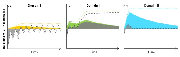
Figure 2
In contrast, improving a severely degraded ecosystem under adverse environmental conditions (Domain I in Figure 1b) is expensive and takes longer to materialise (grey line and area in Figure 2a). Here, we illustrate a case in which site preparation did not immediately result in vegetation improvement but disturbed the existing vegetation and led to an initial decline in vegetation cover. This decline implies a lack of benefits in the first years even with additional maintenance (see early negative values of grey line and area in Figure 2a). As ecosystems tend to return to the lower stable equilibrium (i.e. degrade) if situated above the lower branch of the hysteresis curve in Domain I, recurrent maintenance costs arise (resulting in repeated sharp decline in grey line in Figure 2a), as in Domain II. In the case depicted in Figure 2a, maintenance costs are exemplified to occur every other year (repeated sharp decline in grey line in Figure 2a) reflecting variability in rainfall and vegetation establishment. However, such investments to sustainably improve a degraded ecosystem may not be economical as shown by both total negative present and future net benefits (grey line and area in Figure 2a).
Investment in a healthy ecosystem that tends to improve naturally (located below the upper branch of the hysteresis curve in Domain III, Figure 1b) can increase the speed of improvement (pronounced slope in light blue line and area in Figure 2c), usually at modest investment cost. Net benefits only arise at an early stage and vanish once the ecosystem would have reached the healthy stable equilibrium without the intervention (grey line and area in Figure 2c). The healthy stable equilibrium that is reached will be the same with and without investment. Here, the acceleration of restoration as the ecosystem develops towards the higher stable equilibrium (healthy regime) needs to be high enough to render investment attractive.
SLM as a preventive measure has in the long run frequently been found to be cheaper than ecosystem restoration (ELD 2015, Nkonya et al. 2016). However, investment costs need to be considered in conjunction with expected benefits, risk of failure and the passage of thresholds, meaning that higher upfront costs might in the long run be offset by restoration benefits (Zahawi et al. 2014, Gilardelli et al. 2016). Long-term field experiments with controlled management and environmental conditions are crucial to test and refine important ecosystem properties and feedbacks captured in models to advance existing and build new theories and inform decision making (Foster et al. 2016). They are key for improving our often incomplete knowledge about the socio-ecological dynamics that facilitate or constrain the implementation of specific land use strategies (Sietz and Van Dijk 2015) and evaluating threshold behaviour (Suding and Hobbs 2009). This is a pre-requisite for land-based management decisions that are well-suited to address heterogeneity in global sustainability challenges such as loss of biosphere integrity, livelihood insecurity and socio-ecological vulnerability (Sietz 2014, Steffen et al. 2015, Kok et al. 2016).
In the face of ever-present uncertainty, learning through monitoring of key processes and feedbacks, scenario analysis and adaptive management is central for decision making and inherently linked to resilience thinking. Efforts aimed at increasing response diversity may be particularly beneficial to address uncertainty in future disturbances and environmental conditions (Suding and Hobbs 2009). Response diversity describes the variety and heterogeneity of species, ecological communities and feedbacks but also managerial processes, allowing ecosystems and human flexibility to respond in various ways and prepare for anticipated effects of disturbances and ongoing change. High response diversity enables some system components or functions to persist, recuperate or transform when disturbed, while others may experience damage or vanish. Further, as costs and benefits associated with alternative ecosystem regimes can differ significantly depending on land users’ perceptions, demands and expectations (James et al. 2015, Tarrason et al. 2016), stakeholder involvement is paramount in decision making.
Note: For full references to papers quoted in this article see