Introduction

A generally accepted framework for the description of catastrophic shifts is that of the fold catastrophe (Figure 3). In this framework, certain disturbances caused by unfavourable external conditions can cause the system to shift towards a degraded state. The maximum disturbance that can be absorbed by the system is the system’s resilience. As long as the disturbance stays within the resilience, the system has the capacity to return to its previous conserved state when the disturbance ceases. As the figure shows, resilience decreases when the system approaches the tipping point. Knowing the exact magnitude of the system’s resilience a priori is rather challenging, as it usually depends on feedback loops between biotic and abiotic components of the ecosystem.

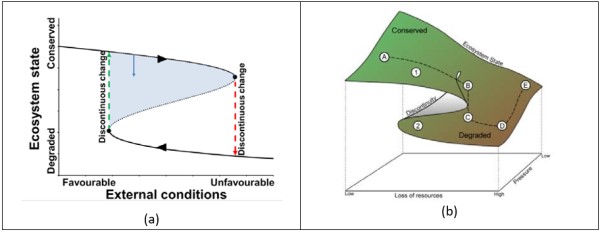
Figure 3

When the system’s resilience is exceeded, the system jumps to a new state through a sudden shift when the tipping point is passed. Note that the term ‘sudden’ can be misleading as humans have the tendency to relate human timescales to their perception, thereby relating sudden ecosystem shifts to perhaps weeks or months. However, the term ‘sudden’ can have a much broader time range. For example, de Menocal found in 2000, that the transition of the Saharan region from annual grasses and shrubs to desert conditions took around 500-600 years, while Scheffer et al. (1993) recorded that transitions between two stable states in shallow lakes can take between 1 and 5 years. The range in duration of an ecosystem shift, depends on the size and nature of the ecosystem. ‘Sudden’ should also be interpreted in relation to the rate of change of the main driver the ecosystem responds to (such as change in rainfall). Shifts can take place over different timescales ranging from days to years, and, for example, a slow ecological change may precipitate an abrupt economic change.

The degraded state may be stable in the sense that it also presents a new resilience against external conditions. If the ecosystem is governed by one important external variable, then restoration via this variable ultimately leads to a recovery of the system via another path (see Figure 3, ‘D’ to ‘E’).

In practice however, the system may not return to the initial state but will instead lead to an alternative situation. The reason is that the shift from the original state to the degraded state is often accompanied by a loss of other resources, and that the restoration attempt does not affect these resources in such a way that a shift back to the original desirable state happens. Especially for dryland systems, the absence of a resource may prevent transition to a conserved state. This alternative situation is not always desirable as it may hold inferior ecosystem value than the initial system. This can be illustrated as a cusp catastrophe (Figure 3B), which is a 3-D version of Figure 3A, and in which separate axes are used for pressure and loss of resources.

In Figure 3B, (A) represents an area where a driver is causing pressure to the ecosystem which nevertheless retains a good status and high resources. Here the system is in stable state 1, and can maintain this state regardless of pressure (e.g. grazing) due to its resilience. As resources become depleted the system reaches a region where two alternative stable states (1 and 2) coexist. When the resource depletion has brought the system to the tipping point (B), it shifts to state (C). An example is a grazing system where the rate of consumption gradually grows and at a certain moment exceeds the rate of biomass production leading to a collapse. If resources are depleted further (D), transition back to (C) may require some kind of effort with respect to the lost resources. Going back to state (B) is even more difficult (as explained for Figure 3A). More importantly, eliminating the exerted pressure drives the system to an alternative state (E) rather than back to its pristine condition, because the depletion of resources and not the (grazing) pressure was driving the collapse. Therefore, it is possible that the system becomes “trapped” in this alternative state, especially if resources at hand are non-renewable (e.g. soil) and their loss cannot be amended within a reasonable timeframe (e.g. the human lifespan).

The cusp catastrophe concept and variations can be adopted for different ecosystems or selected ecosystem health indicators. For example, similar transitions can take place between different states of a forest where the combined high fire frequency and loss of resources (e.g. seed bank or soil) can lead to changes in the phenology of the vegetation and ultimately to a stable shrub land. As long as resources do not recover the system would remain locked in this state. However, when resources start to recover, a gradual improvement of the ecosystem would occur according to Figure 3B. Comparable to grazing, at higher fire frequencies the cusp model predicts hysteresis.

CASCADE's results

Although CASCADE’s field sites include different Mediterranean ecosystems, in general the plant communities in the degraded situations are very different from the respective healthy references both in composition and abundance (Valdecantos and Vallejo 2015, Valdecantos et al 2016). Pressure resulted in more homogeneous communities than in undisturbed states, except in Randi and Castelsaraceno, with little variations within degradation levels.

The field sites affected by grazing pressure showed a general decrease in plant diversity with grazing pressure and, hence, can be described as overgrazed. In addition to these change in diversity, we observed a profound change in species composition in all grazed sites, more modest in Castelsaraceno. Aboveground biomass was reduced in two out of three grazed sites (Castelsaraceno overgrazed and Randi) but increased in Messara. Plant spatial pattern and distribution in the grazed states is markedly different than in the un-grazed ones, with higher cover of open areas and lower length and width of the plant patches in the grazed plots. These changes reduce the resource sink capacity as observed in other areas subjected to grazing and, hence, resource conservation. Similarly, LFA derived indices (infiltration, stability and nutrient cycling) are lower in all degraded sites than in their respective references suggesting a degradation of soil surface conditions and, thus, soil, water and nutrient conservation in the system. On the other hand, grazing, especially when intense, represents an important tool to reduce fire risk in areas with prolonged drought periods by reducing the amount of fuel available. In these cases, grazing systems provide another service to people as they reduce the fire hazard.

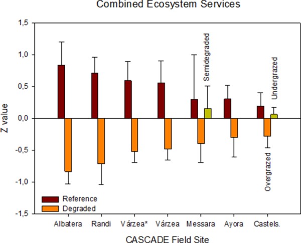
Figure 4

The sites affected by fire pressure offer two complementary pictures of secondary succession after wildfires: a very initial stage of vegetation recovery in Várzea and a mature continuous shrubland without tree- canopy recovery in Ayora. In the short term, the ecosystem shows important reduction in species richness, biomass, vegetation patches, stability, infiltration and nutrient cycling. These result in an overall significant loss of ecosystem services (Figure 3). But this maritime pine forest ecosystem has the ability to recover with time most of them, if not all. Thirty-five years after the fire, the Ayora burned areas recovered ecosystem functionality to values of the Reference pine forest, and showed a spatial arrangement of vegetation that better conserves the resources, and accumulated similar amounts of understory and belowground biomass and litter. Pine regeneration after fire, and hence catastrophic shifts, depends on many factors such as fire-interval, pre-fire basal area, slope aspect, land use history or competition with grasses at the seedling stage. The scarce presence of pines in the Degraded states of Ayora field site resulted in a significant reduction of the C sequestration service and could be improved by appropriate post-fire management. The observed shift from forest to non-forest (shrubland) vegetation observed in Ayora is not uncommon especially in drylands and is likely to occur in the very high fire recurrence of the Degraded plots in Várzea. The short interval between the two latest fires (2005 and 2012) may cause the change from forest to non-forest vegetation in this area as the time for the first flowering in Pinus pinaster may take between 4 and 10 years. This imbalance between fire regime and dominant plant species’ life histories or unfavourable post-fire conditions may result in a failure to recover pre-fire carbon stocks and hence C sequestration service. Stephens et al. (2013) suggested that this shift might not be catastrophic but would affect most ecosystem services. All ecosystem services showed significant short-term losses after the fire (Várzea) but only biodiversity and C sequestration losses lasted in the long term (Ayora).

Albatera showed the highest relative losses of all individual ecosystem services of all CASCADE field sites (Figure 4). It is the most stressed site as reflected by the very low aridity index (0.16) and multiple diffuse pressures that are and have been acting in the place for long. The main ecosystem properties affected by degradation were those related to the spatial distribution of vegetation and open areas (sink/source spatial pattern) that finally determine the conservation of resources. The Degraded landscape showed a reduction of vegetation cover, with less and smaller patches of vegetation at longer distances from each other, and higher proportion of bare soil, which in turn reduces capacity of water infiltration and nutrient cycling, and decreases water conservation and soil conservation, and, finally, reduces productivity (Boeschoten, 2013).

Biodiversity was also highly reduced in the degraded areas probably related to the absence of tall shrubs that act as keystone species in these semiarid shrublands (Maestre and Cortina, 2004). The stability index showed the lowest loss in the Degraded as compared to the Reference state. Previous works in semiarid Mediterranean areas have shown that the stability index is less sensitive than the other LFA indices to detect differences between land uses and/or degradation levels (Mayor and Bautista, 2012). López et al. (2013) found lower values of the LFA stability index as degradation increased associated to lower vegetation cover and patch density, length and width, but a further increase of the index with more intense degradation as the exposed rock surface is higher and the sediments susceptible to be transported is lower. These results could therefore suggest that the system might have passed a threshold of irreversibility.

Ecosystem services have shown important losses due to grazing in the order Randi > Messara > Castelsaraceno (Figure 4) following a decreasing order of aridity. Wang et al. (2014) established 0.32 as the threshold value of the aridity index that determines net N losses or accumulations. Castelsaraceno and Randi are well above and below this value of aridity, respectively, while Messara is around this threshold.

Discussion and Conclusions

Results showed that degradation pressures severely impacted ecosystem properties and services of the selected ecosystems along the Mediterranean basin in a wide range of ecological, biogeographical and historical characteristics. The higher the aridity, the higher the loss of ecosystem services. Some observed changes from the reference towards the degraded states, suggest that certain degradation thresholds might have been passed. Sudden ecosystem shifts in Mediterranean ecosystems are therefore transitions that result in decreased plant cover and diversity, accompanied by increased loss of resources and reduced delivery of ecosystem services.