| Authors: | Tsanis, I. K. and Daliakopoulos, I. N. |
| Editor: | Jane Brandt |
| Source document: | Daliakopoulos, I. and Tsanis, I. (eds) 2014. Drivers of change in the study sites. CASCADE Project Deliverable 2.2. CASCADE Report 06. 59 pp. |
Climate datasets
Climate model data were obtained from 9 GCMs of the 5th phase of the Coupled Model Intercomparison Project (CMIP5 - Taylor et al., 2012). The simulations are based on the future emission scenarios as they are defined by specific Representative Concentration Pathways (RCPs - Moss et al., 2010). The RCPs are based on the change in the radiative forcing (ΔW/m²) due to the application of various Shared Socioeconomic Pathways (SSPs). Here we focus on 3 such RCPs, namely RCP2.6, RCP4.5 and RCP8.5 taking after the projected change in the radiative forcing to be posed in the earth atmosphere (2.6 W/m², 4.5 W/m², and 8.5 W/m² respectively) by the end of the 21st century. The model data have been previously used to assess drought propagation at regional level (Vrochidou et al., 2013) and global scale (van Huijgevoort et al., 2014). Here we focus on a domain that spreads between latitude 34°N to 44°N and longitude 10°W to 35°E that includes the entire European Mediterranean and all the CASCADE Study Sites.
Table: List of the CMIP5 GCMs that were used to provide the temperature and precipitation data.
| Modeling Center | Model | Institution |
| CCCma | CanCM4 | Canadian Centre for Climate Modelling and Analysis |
| CNRM-CERFACS | CNRM-CM5 | Centre National de Recherches Meteorologiques / Centre Europeen de Recherche et Formation Avancees en Calcul Scientifique |
| CSIRO-QCCCE | CSIRO-Mk3.6.0 | Commonwealth Scientific and Industrial Research Organisation in collaboration with the Queensland Climate Change Centre of Excellence |
| EC-EARTH | EC-EARTH | EC-EARTH consortium |
| IPSL | IPSL-CM5A-MR | Institut Pierre-Simon Laplace |
| MIROC | MIROC-ESM | Japan Agency for Marine-Earth Science and Technology, Atmosphere and Ocean Research Institute (The University of Tokyo), and National Institute for Environmental Studies |
| MOHC | HadGEM2-ES | Met Office Hadley Centre (additional HadGEM2-ES realizations contributed by Instituto Nacional de Pesquisas Espaciais) |
| MPI-M | MPI-ESM-MR | Max Planck Institute for Meteorology (MPI-M) |
| NASA GISS | GISS-E2-R | NASA Goddard Institute for Space Studies |
Raw climate model outputs cannot be used in their native form in climate change impact studies, due to the high systematic errors and biases that they feature. Methods of statistical bias correction are increasingly being developed and adopted as means to translate climate model projections into actual impacts. These methods involve some form of transfer function, or other techniques for equalization of statistical characteristics between modeled and observed variables.
Raw climate model outputs cannot be used in their native form in climate change impact studies, due to the high systematic errors and biases that they feature (Leander and Buishand, 2007; Sharma et al., 2007; Wood et al., 2004). Methods of statistical bias correction are increasingly being developed and adopted as means to translate climate model projections into actual impacts. These methods involve some form of transfer function (Block et al., 2009; Déqué, 2007; Fowler et al., 2007; Grillakis et al., 2013; Piani et al., 2010), or other techniques for equalization of statistical characteristics between modeled and observed variables (Engen-Skaugen, 2007; Horton et al., 2006; Leander et al., 2008; Leander and Buishand, 2007).
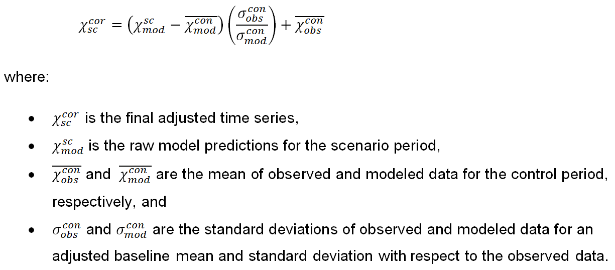
Here we use a widely used bias correction method presented by Haerter et al. (2011) to correct the monthly precipitation and temperature data for biases in mean and variance. The bias in mean is corrected by subtraction of the differences found between observed and modeled values and a correction to the model data is applied to conform to the variability of the historical data. This procedure takes the sequence of anomalies and scales them consistently with the observed historical variability. In the case where data follow the normal distribution the transfer function is linear and is of the form:
The methodology is applied for each calendar month in order to cope with the correction in the precipitation seasonality. The E-OBS gridded data set (Hofstra et al., 2009) was used as observational dataset to correct the climate model data for their biases both in temperature and precipitation.
Vegetation yield
FAO has addressed the relationship between crop yield and water using a simple equation (Doorenbos and Kassam, 1979) where relative yield reduction is related to the corresponding relative reduction in ET:
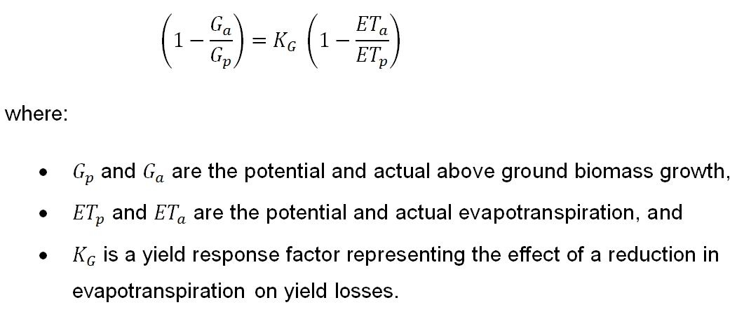
The yield response factor KG captures the essence of the complex linkages between crop production and water use (Doorenbos and Kassam, 1979). Equation 2 is a water production function which has shown a remarkable validity at basin scale, field scale (Yacoubi et al., 2010), and in decision support systems (Gastélum et al., 2009) and can be applied to all agricultural crops, i.e. herbaceous, trees and vines. It is noteworthy that for particular values of KG (e.g. alfalfa, bananas and peas with KG>1), and small values of ETa/ETp denoting water stress, the ratio Ga/Gp can become negative, implying that the production of crops is not possible.
Numerous empirical and physically based models have been constructed in order to derive ETp and /ETa values. Aiming to simplify without much error, the method proposed by Turk (1961) and later verified (e.g. Liang, 1982) can be used to estimate the annual ETa as
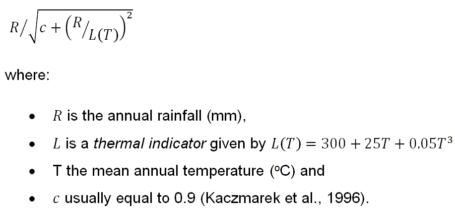
Furthermore, the Blaney-Criddle formula (Blaney and Criddle, 1962) requires mean daily temperature T and the mean daily percentage p of total daytime hours, both on a monthly basis, in order to derive daily ETp as p(0.46T+8). Value of p can be estimated or derived from tables (Doorenbos and Pruitt, 1975) and ETp can be aggregated to produce long term averages.
Vegetation stress
Despite the considerable uncertainties in the future climate drivers (Koutroulis et al., 2013), temperature increase due to climate change is considered a certainty in the peer-reviewed literature (Parry et al., 2007), with authors questioning not "whether" but rather "when" certain thresholds will be exceeded. Joshi et al. (2011), suggest that while a global average 2°C warming threshold is unlikely to be passed before 2060 for all greenhouse-gas emission scenarios, on regional scales, this threshold will probably be exceeded by 2040 if emissions continue to increase. This projected temperature increase will imply higher evaporation and drier conditions under equal or less rainfall (AWC and WWC, 2009). A recent IPCC report (Bates et al., 2008) predicts that climate change over the next century will also affect rainfall patterns, reducing its frequency and increasing its intensity. While changes differ strongly across models and some areas are projected to experience increased precipitation (Marchal et al., 2011), many parts will experience a decline in precipitation. Concerning many parts of the arid regions, precipitation is expected to decrease by 20% or more over the next century (AWC and WWC, 2009). Agriculture and food security are threatened by these changes, as an increase of T with a parallel decrease or even stationarity of P leads to a decrease of the ETa/ETp fraction and therefore to a reduction of the expected Ga. This decrease in the potential crop yields and the productivity of water in agriculture with high temperatures has been previously predicted (Cline, 2007; Kundzewicz et al., 2007) and is expected to cause an increase in the demand of the already reduced supply of agricultural water (Döll, 2002).
Detecting trends and seasonal changes of vegetation related time series may enable the classification of these changes: changes in the trend component often indicate disturbances, while changes in the seasonality may indicate phonological changes (Verbesselt et al., 2010a, 2010b). Several generic change detections approaches have been proposed, e.g. by Lavielle (1999), Adams and MacKay (2007) and (Verbesselt et al., 2010b) after Haywood and Randall (2008). Here we estimate the variance change points of the NDVI timeseries using the method of Lavielle (1999). The method assumes that the data follows a normal distribution and detects simultaneous changes in the mean and variable of the distribution but requires no assumptions about the dependence structure of the time series. After the detection of breaks, the NDVI time series for each of the Study Sites is split into a seasonal and trend component and compared against events and behaviors that may have disturbed the system in some way (e.g. fire, drought, land use change). While trends are easier to detect and attribute to a persistent driver, phonological events are difficult to precisely identify with remote sensing images, so researchers tend to prefer arbitrary classifications (e.g. Eastman et al., 2013). Here we make two main assumptions following Lu et al. (2003) and Prabakaran et al. (2013). The first is that land covers dominated by shrubs and herbaceous vegetation or crops that follow an annual cycle are responsible for the seasonal NDVI signal while land dominated by woody and evergreen vegetation is mainly responsible for the deseasonalised signal. The second assumption is that deciduous forests display an earlier onset of greenness, followed by evergreen forests.
Grazing
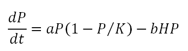
The predator-prey system (Noy-Meir, 1975) typically serves as a basis for models that describe the dynamics of grazing systems. The rate of change of the harvested biomass P (standing crop) is represented by the differential equation:
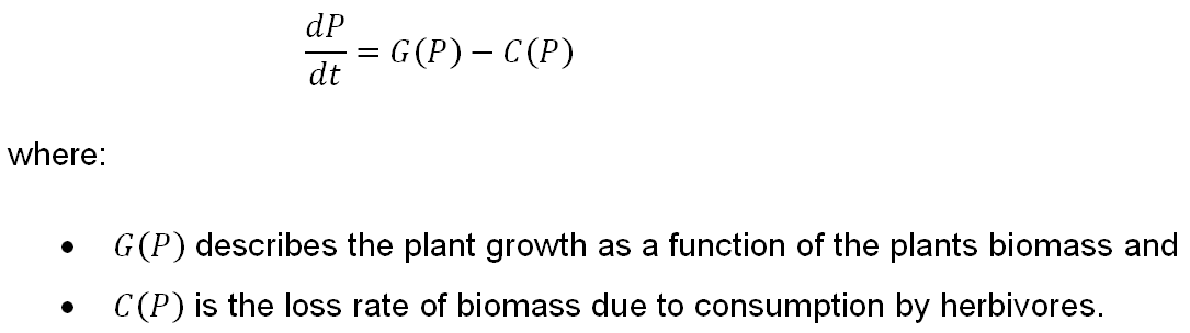
G(P) is commonly given by the logistic growth equation G(P)=aP(1-P⁄K), where a is the plant growth coefficient (the intrinsic growth rate) and K the carrying capacity of the land (the maximum amount of resource stock when there is no harvest activity). From the G(P) equation it is inferred that the relative natural growth G(P)⁄P is a linear function of the biomass level P and approaches its maximum, equal to a, when P approaches zero. Parameter a is mainly related to the actual species under observation while K depends mainly on the natural environment of the stock, such as size and biological productivity of the habitat.
According to the Gordon Schaefer model (Schaefer, 1957), losses due to grazing can be considered proportional to both biomass (relies on the existing stock of renewable resource at a given period) and herbivore density, giving C(P)=bHP, where b is the biomass consumption coefficient. It can be argued that the land's carrying capacity K and plant growth coefficient a are related to the soil quality and the climate conditions, meaning that these parameters are under stress in arid areas. The same is not true for grazing, as the consumption coefficient b possibly increases as nutritional needs may change under pressure (Ayres, 1993; Robbins et al., 1987) and herbivores can be quite effective at grazing.
Following from the above, the rate of change of the harvested biomass P from Equation 1 can be written:
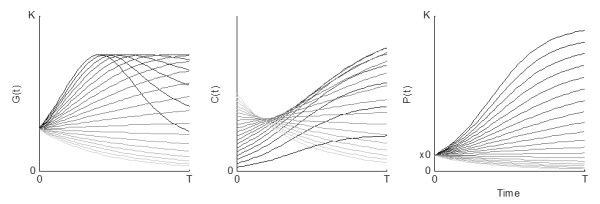
For G(P)>C(P) the natural growth of the resource is greater than the harvest amount. As a result, the resource stock P will increase. The result is opposite when the harvest amount exceeds the natural growth of the resource. The figure below shows vegetation growth and consumption for a system with initial biomass x0, plotted against time. The effect of increasing herbivore densities on the system is depicted with lighter lines.
Equation 4 can reach two possible states of equilibria (dP⁄dt=0). If P(t)=0 then the vegetation resource has been depleted, eventually leading to the reduction of soil services along the mechanisms of the desertification paradigm downward spiral (Adeel et al., 2005; Hassan et al., 2005). On the other hand, sustainable use also implies that the net biomass production is zero but this time the ecosystem can maintain a steady level of biomass stock, such that:
Solving Equation 5 for P, we get P=(a-bH) K⁄a which means that the biomass and eventually the growth rate comprises a function of H. If the vegetation growth does indeed follow the logistic function for growth then the maximum vegetation biomass yield is equal to aK⁄4, also called Maximum Sustainable Yield (MSY), at which point the herbivore density is equal to a⁄2b. Keeping all other parameters stable along the MSY path, as the herbivores density H increases the biomass production rate can be insufficient to cover it until H reaches the critical value a⁄b and the system deteriorates.
Substituting Gp with the logistic growth equation, Equation 2 can be transformed to:
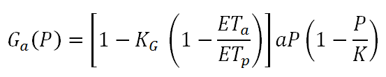
which infers that Ga is maximized as ETa approaches ETp. Taking into account the effect of climate on vegetation growth and assuming zero net biomass production, Equation 6 is transformed to:
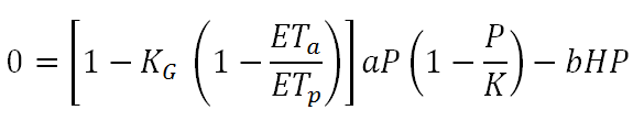
As in Equation 5, the maximum vegetation biomass yield is again equal to aK⁄4 but this time it is achieved for H=[1-KG (1- ETa/ETp) ] a⁄2b, so it is also related to climatic conditions (Daliakopoulos and Tsanis, 2014). Based on these empirical relationships, a robust qualitative concept of resilience emerges. While modeling within CASCADE may follow a more quantitative approach, this concept roughly explains the principals of the interaction between vegetation, climate and herbivores. Similar concepts are described by Jeltsch et al. (2014) and Rietkerk et al. (1997, 1996).
References
See the full report for details of all the other work cited on this page